Greenhouse Gas Flux Monitoring for Finland
The greenhouse gas monitoring system developed at the Finnish Meteorological Institute quantifies CO₂ and CH₄ fluxes regionally in Finland with high resolution (0.1°-0.2° lat x lon) and globally with lower resolution (up to 1° lat x lon). Integrating bottom-up flux estimates with atmospheric measurements, the system tracks emissions and their changes to assess the effectiveness of mitigation efforts.
Our greenhouse gas monitoring system consists of both bottom-up and top-down estimates. Bottom-up methods start from individual sources and scale up using scientific knowledge, for example, through inventory calculations or process-based models, to estimate greenhouse gas emissions for a sector or region. Top-down methods, on the other hand, use measurements of CO₂ and CH₄ in the atmosphere from ground-based towers or satellites and combine them with models of atmospheric circulation to infer where the emissions originated. These top-down methods, also called atmospheric inverse models, use bottom-up estimates as a starting point to help constrain the mathematical problem they aim to solve.
The main components developed by FMI for the greenhouse gas monitoring system are JSBACH-HIMMELI, which simulates land fluxes, and the inversion model systems CIF-FLEXPART-FMI and CTDAS-FMI, which estimate the fluxes from all sources. The sources include, in addition to land fluxes, the anthropogenic emissions, fire emissions, ocean fluxes and atmospheric sink of methane, to name the most important ones.
Content
- Modelling of greenhouse gas emissions
- Land ecosystem process model JSBACH-HIMMELI
- Atmospheric inverse model CIF-FLEXPART-FMI
- What do we see from the greenhouse gas emission estimates?
- Key publications
- Contact information
Modelling of greenhouse gas emissions
A model represents a real-world system in a simplified yet comprehensive way by formulating its key features mathematically. Modelling of greenhouse gas fluxes is inherently dependent on observations: similar to scientific theory, we cannot confirm whether a model is correct without real-world observations. However, once validated, models estimating greenhouse gas fluxes enable us to extend research beyond what can be studied solely through observations. For example, they allow us to simulate current conditions, such as wetland CH₄ emissions across the entire Arctic, as well as explore how these emissions may change in the future under different climate scenarios. In addition, models can help interpret observations: what could be the processes that control the observed greenhouse gas fluxes?
Land ecosystem process model JSBACH-HIMMELI
JSBACH‑HIMMELI is an ecosystem process model that simulates how land ecosystems exchange CO₂ and CH₄ with the atmosphere. It uses equations that represent the biological, chemical, and physical processes controlling greenhouse gas emissions and can be applied at scales from individual sites to the global domain. JSBACH‑HIMMELI consists of two major components: JSBACH provides the land‑surface backbone for CO₂ exchange, i.e., photosynthesis and respiration, constrained by vegetation phenology, and soil carbon cycling. HIMMELI adds explicit peatland CH₄ balance processes. It uses the JSBACH output to simulate methane production from anoxic soil respiration, methane oxidation, diffusion through the peat column, plant‑mediated methane transport, and the division between oxic and anoxic soil layers, which is determined by water table depth.
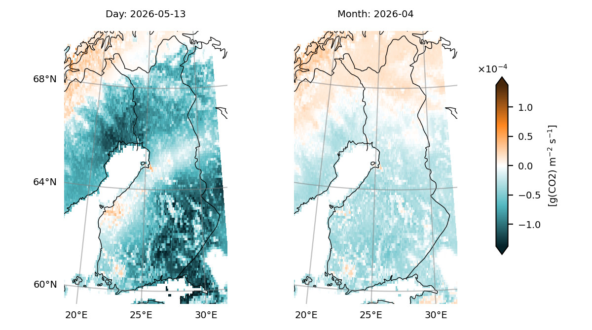
The inputs to JSBACH-HIMMELI include land cover maps, which are often static, and atmospheric variables, such as air temperature, wind speed, solar radiation, air humidity, precipitation, and atmospheric CO₂ concentration, which can be obtained from reanalysis data that is updated with a relatively short time lag of a couple of days. Therefore, we can also obtain process-model based greenhouse gas flux estimates with a lag of a week. With this, we can study timely issues, for example, how a warm autumn affected the CO₂ and CH₄ emissions from Finland’s peatlands in 2025. However, as the modelling results are dependent on the meteorological data used, any biases in these datasets can also cause biases in the greenhouse gas emission estimates. The reanalysis of meteorological fields relies on observations of which some become available only after a while. Thus, using updated meteorological data relying on more observations also gives us more reliable greenhouse gas emission estimates. Similar to many operational data products, the near-real-time estimates serve as our best estimate at the time, and later added information can change the greenhouse gas budgets.
Atmospheric inverse model CIF-FLEXPART-FMI
The Community Inversion Framework (CIF) is a modular open‑source system designed to interface with multiple atmospheric transport models and inversion schemes. We apply CIF’s four‑dimensional variational (4DVAR) optimization scheme while atmospheric transport is simulated with FLEXPART, which represents dispersion and turbulent mixing through virtual particles.
The atmospheric inverse models rely on atmospheric greenhouse gas concentration measurements. First, an initial estimate of spatially distributed greenhouse gas fluxes (prior fluxes) is provided to a three-dimensional atmospheric transport model that simulates how greenhouse gases are transported through the atmosphere. The resulting modelled concentrations are then compared to measurements. When a mismatch between the modelled and measured atmospheric greenhouse gas concentrations is found, the inverse model adjusts the prior fluxes using Bayesian statistics, answering the question: "What are the most probable greenhouse gas fluxes given the atmospheric observations, prior information, and their corresponding uncertainties?"
The concentration of greenhouse gases in the atmosphere depends both on the background concentration and the part that is caused by recent emissions. Background concentration refers to a relatively well-mixed atmosphere, and it is the sum of the past emissions and sinks, i.e., the part of the emissions that remained in the atmosphere. We can measure the accumulated greenhouse gases at measurement sites that are often called “background sites”. They are in remote areas where there are no local large greenhouse gas sources, and thus, they can be used to constrain the large-scale emissions.
The other component in the atmospheric greenhouse gas concentration comes from recent emissions. Based on the modelled transportation of air masses (including the greenhouse gas molecules), we can estimate where the emissions or sinks of greenhouse gas molecules occurred. For the interest of regional emissions, the site-level measurements are taken from higher up in the atmosphere (around 100 m or on top of a mountain) where the air is well-mixed and holds greenhouse gas molecules from a wider area. In addition to these “surface” observations, measurements from remote-sensing satellites can be used. They measure the whole atmospheric column, i.e., the average of the greenhouse gas concentration from the surface level to the top of the atmosphere. Thus, they are less sensitive to the emissions happening at the surface level, but they have superior spatial resolution compared to site-level measurements.
The measured greenhouse gas concentrations include information from all sources and sinks, including land ecosystems and anthropogenic emissions. The sum of all sources and sinks is called “the total budget”. To distinguish between different sources and sinks, we are using the assumed distribution of emissions from each sector, both in time and space. There are also other methods that can be used to partition different sectors (e.g., greenhouse gas isotopologues), but those are not used here.
In addition to meteorological fields, atmospheric observations of greenhouse gas concentrations are required to run the model. Currently, these observations are shared with varying time lags. For example, the European greenhouse gas measurement infrastructure ICOS provides near-real-time observations from many of its atmospheric stations. Globally, observations are available, e.g., from NOAA Obspack or WMO/WDCGG database, and they have their specific update frequencies (not near-real-time). Even if a regional inverse model primarily uses atmospheric observations within the study region, it still needs “background concentrations”, i.e., knowledge of greenhouse gas concentrations at the border of the region domain. So, the global measurements are also needed to constrain emissions within a region. Satellite total column measurements, such as data from Sentinel5P-TROPOMI, are available near-real-time and have a global coverage. However, before those measurements can be used in the inverse model, they need to be processed for inversions, which causes a delay.
What do we see from the greenhouse gas emission estimates?
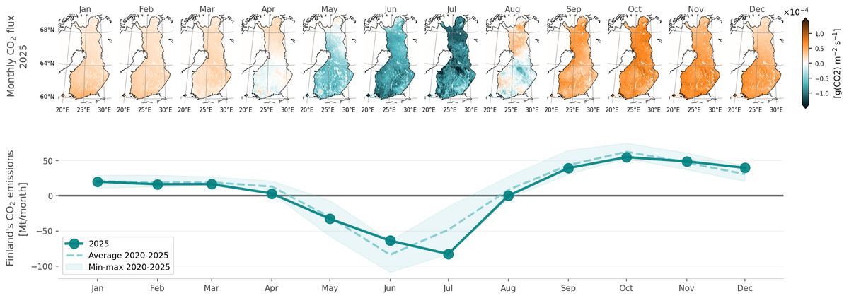
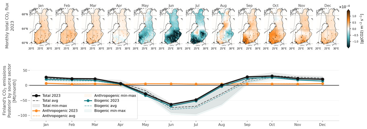
Anthropogenic emissions (both CO₂ and CH₄) have much less pronounced seasonality than land-ecosystem emissions. Thus, the seasonality of the total greenhouse gas budgets is also determined by the land-ecosystem emissions’ seasonality. Based on JSBACH-HIMMELI and CIF-FLEXPART-FMI, land ecosystems in Finland are a net source of CO₂ from September to March on a monthly level. In April and August, the northern part of Finland is a net source but photosynthesis in the southern part of Finland already overcomes the respiration. From May to July, almost all of Finland is a net sink.
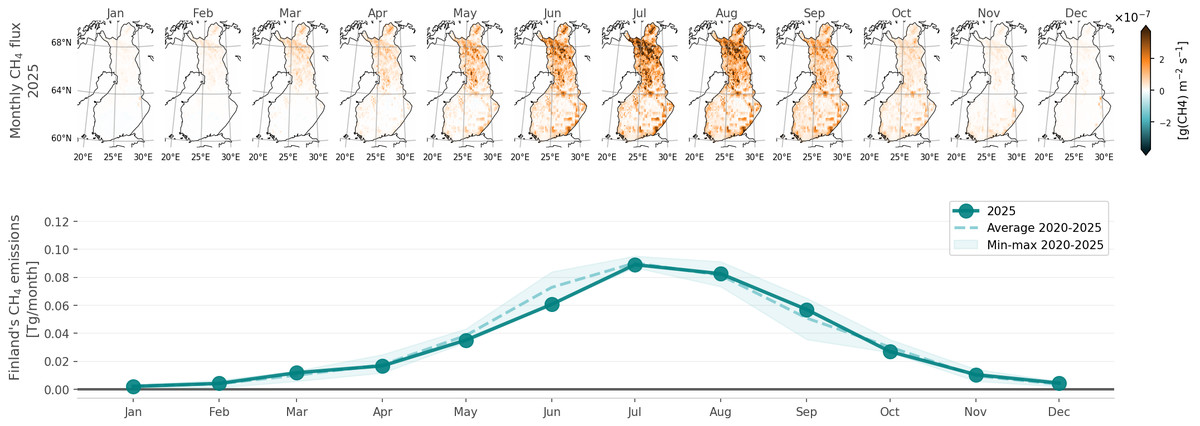
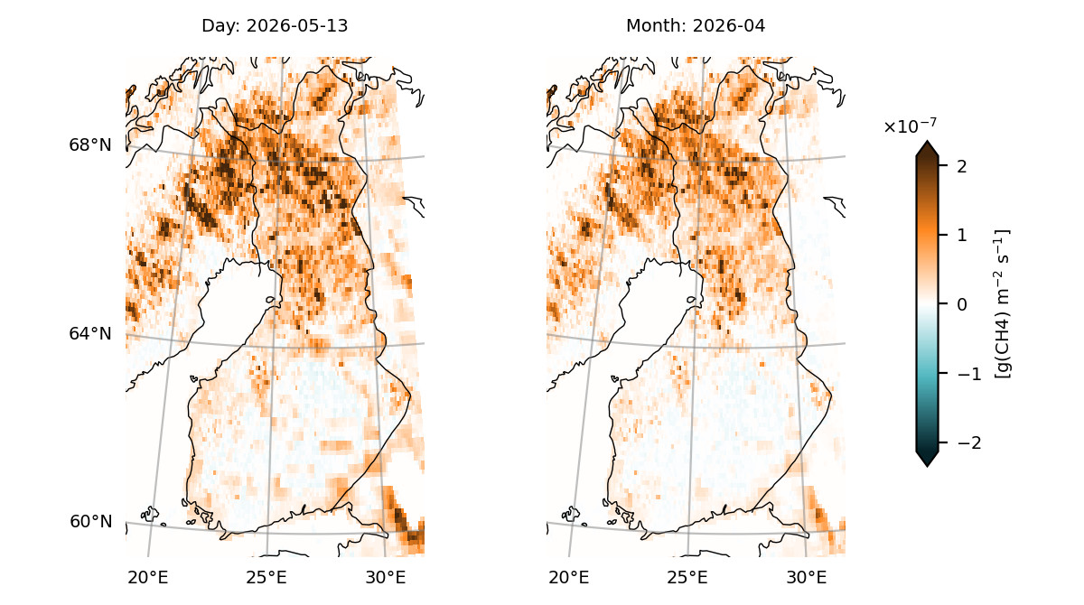
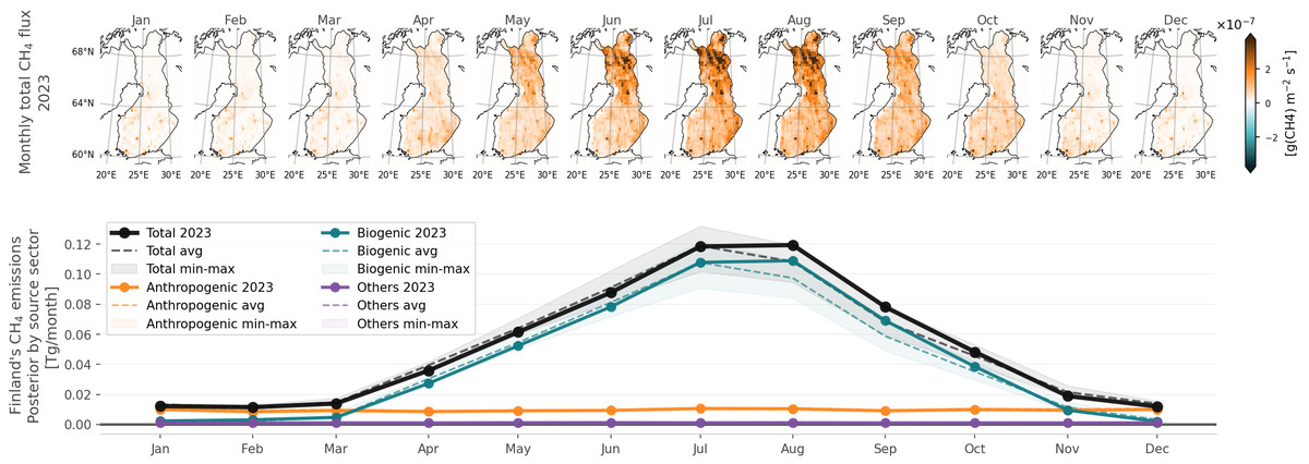
When it comes to CH₄, Finland’s land ecosystems are mostly a net source. This is due to extensive wetland areas in Finland. Both JSBACH-HIMMELI and CIF-FLEXPART-FMI show the highest CH₄ emissions in northern Finland, where the largest pristine peatland areas are located. CH₄ emissions are very small in December to February, start to increase in March, peak in July-August, and then start to decrease in September. The biospheric emissions in CIF-FLEXPART-FMI estimates also include emissions from freshwater systems, which are not included in the JSBACH-HIMMELI estimates. They have similar seasonality to wetland emissions, and most of these emissions originate from southern Finland, which can be seen as a darker orange colour in the map images.
Anthropogenic emissions of CO₂ in Finland are mostly due to energy industries and transport, while most of the anthropogenic CH₄ emissions are from enteric fermentation and manure management of livestock and waste management (Tilastokeskus, national greenhouse gas inventory, 2026), and according to CIF-FLEXPART-FMI model results, they are more prominent in the southern parts of the country.
Key publications
JSBACH-HIMMELI
Petrescu, A. M. R., Peters, G. P., Engelen, R., Houweling, S., Brunner, D., Tsuruta, A., Matthews, B., Patra, P. K., Belikov, D., Thompson, R. L., Höglund-Isaksson, L., Zhang, W., Segers, A. J., Etiope, G., Ciotoli, G., Peylin, P., Chevallier, F., Aalto, T., Andrew, R. M., Bastviken, D., Berchet, A., Broquet, G., Conchedda, G., Dellaert, S. N. C., Denier van der Gon, H., Gütschow, J., Haussaire, J.-M., Lauerwald, R., Markkanen, T., van Peet, J. C. A., Pison, I., Regnier, P., Solum, E., Scholze, M., Tenkanen, M., Tubiello, F. N., van der Werf, G. R., Worden, J. R. (2024). Comparison of observation- and inventory-based methane emissions for eight large global emitters. Earth System Science Data 16: 4325–4350. https://doi.org/10.5194/essd-16-4325-2024
CIF-FLEXPART-FMI
Mengistu, A. G., Tsuruta, A., Berchet, A., Thompson, R., Tenkanen, M., Lindqvist, H., Markkanen, T., Leppänen, A., Laitinen, A., Martinez, A., Fortems-Cheiney, A., Höglund-Isaksson, L., and Aalto, T.: High-resolution inversion of methane emissions over Europe using the Community Inversion Framework and FLEXPART, EGUsphere [preprint], https://doi.org/10.5194/egusphere-2025-5877, 2026.
Berchet, A., Sollum, E., Thompson, R. L., Pison, I., Thanwerdas, J., Broquet, G., Chevallier, F., Aalto, T., Berchet, A., Bergamaschi, P., Brunner, D., Engelen, R., Fortems-Cheiney, A., Gerbig, C., Groot Zwaaftink, C. D., Haussaire, J.-M., Henne, S., Houweling, S., Karstens, U., Kutsch, W. L., Luijkx, I. T., Monteil, G., Palmer, P. I., van Peet, J. C. A., Peters, W., Peylin, P., Potier, E., Rödenbeck, C., Saunois, M., Scholze, M., Tsuruta, A., and Zhao, Y. (2021) The Community Inversion Framework v1.0: a unified system for atmospheric inversion studies, Geosci. Model Dev., 14, 5331–5354, https://doi.org/10.5194/gmd-14-5331-2021.
Contributions
Antti Leppänen (JSBACH-HIMMELI), Anteneh Mengistu (CIF-FLEXPART-FMI), Maria Tenkanen (visualisation, page content).
Contact information
To access the data, please contact Tuula Aalto (tuula.aalto@fmi.fi).
13.5.2026